Paper Replication: High Frequency Trading in a Limit Order Book

This post is a project based off Avellaneda and Stoikov’s 2006 paper High Frequency Trading in a Limit Order Book, which simulates a market-making strategy that sets quotes off an indifference price: an offset to the midprice based on inventory skew. I calibrate the model in Python to sample L2 data from LOBSTER & implement the paper - learning the basics of limit order books and the difficulties of simulating a HFT strat. The code is here.

The idea of this paper is to formulate a mathematical model of market-making based off optimal control and then solve it, yielding an elegant formula for quotes. It is a stylized model that ignores real world complexities like latency, queue position, fees, order types & sizes, adverse selection, etc (hence leading to unrealistic PnL). Regardless, it is still a good learning opportunity for an amateur like me!

Paper Overview

The idea of a market-maker, I learned, is to quote (limit) bid and ask orders on both sides of the order book, get filled and earn the spread repeatedly, while avoiding pitfalls like adverse selection.

Bouchaud in Trades, Quotes & Prices illustrates: if a market-maker quotes a 54.50-55.50 market, an insider knows the company is about to announce a drop in profits and revises his valuation to 45. The insider sees the chance to short sell his stock for profit, and submits market sell orders, hitting the market makers bids. The maker adjusts his bids downwards, but still gets filled and accumulates inventory. At 50, the maker must offload his inventory at a loss.

First, the value function. This is an expected value of wealth under exponential utility.

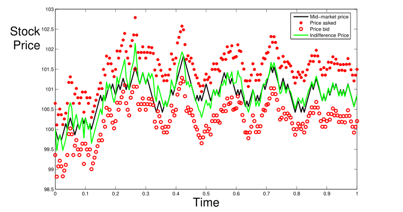
Somehow, the authors use complicated PDE & control theory math (beyond my level) to get

The indifference price is used to generate a symmetric quote of bid and ask that brackets it:

$r$ is the midprice $s$ adjusted by an offset penalty. The offset term scales the inventory $q$ by the product of risk parameter $\gamma$, volatility $\sigma$ and the remaining time till the end of the trading session $T-t$.

The idea is, as inventory $q$ accumulates (say as a result of adverse selection/trending downward prices), the offset term increases, $r$ drops and the quote distances (to $r$) $\delta^b$ and $\delta^a$ are unchanged. Then ask price $P_a$ is more aggressive while $P_b$ is deeper in the book. This causes asks to get lifted more, reducing inventory. Inventory then oscillates back and forth around set point 0. The risk parameter $\gamma$ is in between 0 and 1, and the larger it is, the larger the offsets and smaller the reservation spread, resulting in tighter inventory control.

In the finite horizon case, as $t\rightarrow T$, e.g the trading day ends, the market-maker must clear his inventory. The offset term converges to the midprice, while the quoted spread decreases.

Simulation

The authors then simulate the model on a stationary Brownian motion model of stock prices.

I wanted to adapt the model to historical stock data. So, I went to LOBSTER, fetched the free 1 day (2012-06-21) of L2 book data for AMZN. Now, I needed to decide on parameters. First, $dt$. How often should we quote? I compute the number of price level/queue changes in that day:

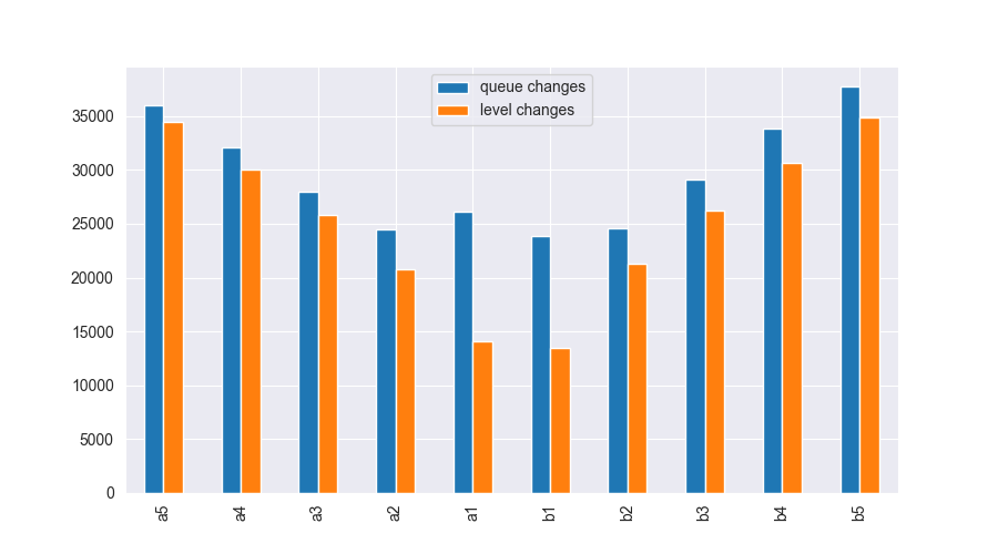
So, 3.3e4/60/60/6.5=1.5. The mean time it takes for a change in queue depth in the fifth best price level is 1.5s.

I settled on 1s. Next, arrival rates. I soon realized backtesting in HFT is not straightforward. This is because of counterfactual outcomes: quoting will add to the book and disturb its original form. In this paper and others, they use Poisson processes to model arrivals.

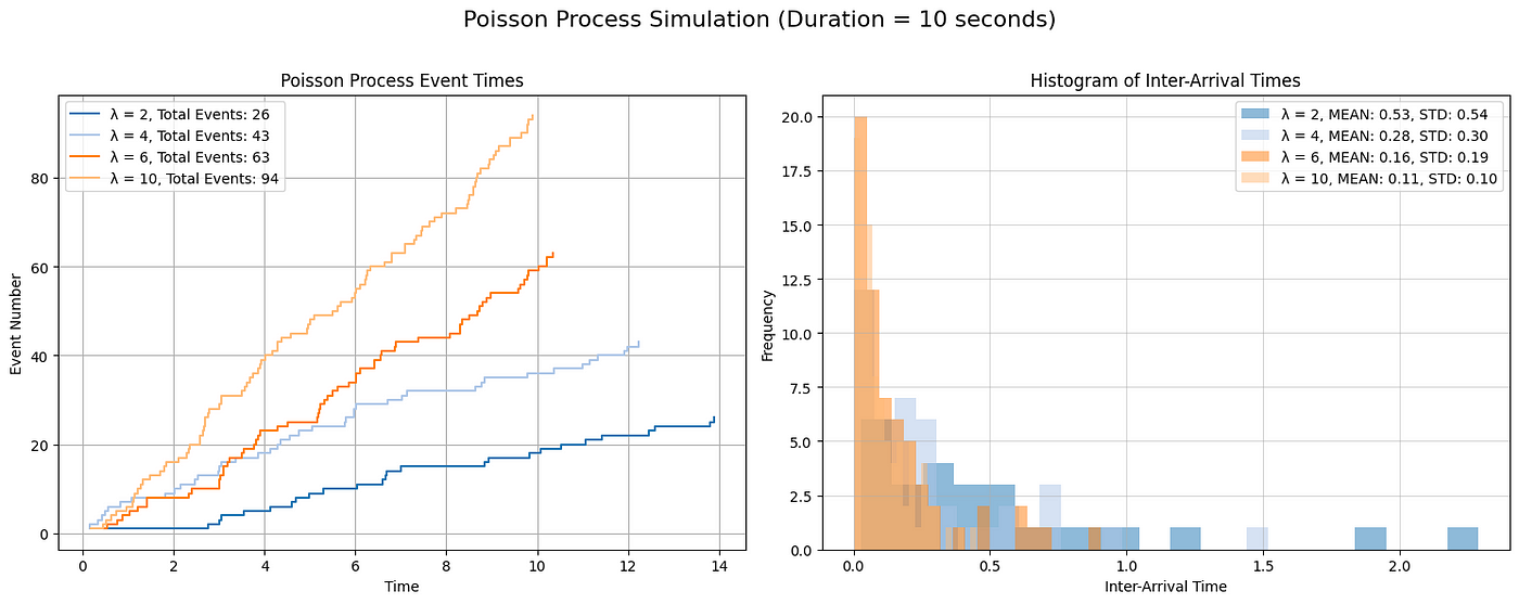
Assuming market orders follow Poisson processes, interarrival times are exponentially distributed. The probability of a quote, say $P_b$, at $\delta_b$ from $s$, getting filled by a market order within $dt$, is an $Exp(\lambda (\delta_b) \space dt)$ random variable with CDF $F(dt) = 1 - e^{\lambda (\delta_b)\cdot dt}$.

$\lambda$ is the rate parameter and $E(dt)=1/\lambda$. This is assumed to be proportional to $\delta$: the further away a quote is from the top of book, the more time it takes to get filled, thus $\lambda$ should be more. The authors use the formula

This means $\lambda$ itself is an exponential function of $\delta$ with constants $A$ and $k$. How should they be computed? The paper does not say, but Lehalle provides the answer in Quant Stackexchange:

The idea is, for a given $\delta P$ to mid, what is the intensity to be hit? For any starting time $t_0$, record midprice, then calculate how long it takes for midprice to move by $\delta_P$. Take the mean under Poisson assumption and $\lambda=1/E(t)$. Pick two distances, then find $A$ and $k$ by this formula:

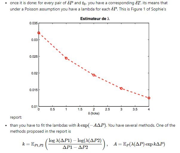
We first need 2 lambdas and two distances from mid to calibrate our curve. We first difference row wise (distance of price level to mid) and calculate quartiles. At 80th percentile, the dist from mid in L5 is $1.55$ and min is $0.05$.

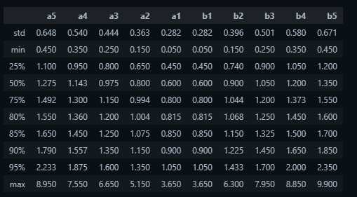
Then, we difference mid and calculate a running sum. Each time our sum exceeds our targets (above), we record the TimeDelta.

def find_marked_time_deltas(arr, d):

    running_sum, last_occurence_time, elapsed_times = 0, None, []
    for time_delta, value in arr.iteritems():
        running_sum += value 
        if abs(running_sum) >= abs(d):        
            if last_occurrence_time is not None:
                elapsed_time = time_delta - last_occurrence_time
                elapsed_times.append(elapsed_time)
            last_occurrence_time = time_delta
            running_sum = 0  

    return pd.Series(elapsed_times).describe([0.25,0.5,0.75,0.8,0.85,0.95])


def calculate_lambdas(df):

    # calculate book width: the distance from mid for all order book events 
    dist = clean_levels.sub(df.mid,axis=0).drop('mid', axis=1).abs()
    dist_quartiles = dist.describe([0.25,0.5,0.75,0.8,0.85,0.9,0.95])
    display(dist)
    upper, lower = dist_quartiles.loc['80%'].max(), 0.15

    # difference midprice
    mid_diff = clean_levels.mid.diff().dropna()
    mid_diff = mid_diff[mid_diff !=0]

    # see function
    upper_times = find_marked_time_deltas(mid_diff, upper)
    lower_times = find_marked_time_deltas(mid_diff, lower)
    u_time = upper_times.loc['mean'] 
    l_time = lower_times.loc['mean']

    u_lambda = 1/u_time.total_seconds()
    l_lambda = 1/l_time.total_seconds()

    return dist, dist_quartiles, u_lambda, l_lambda, upper, lower

def estimate_a_and_k(u_lambda, l_lambda, upper, lower):
    k = np.log(l_lambda/u_lambda)/(upper - lower)
    A = l_lambda * math.exp(k * lower)
    return A, k

For orders sitting at $\delta_1 = 1.55$ and $\delta_2=0.15$ from the mid it takes on average 1m24s and 2s to get a fill. Our lambdas are thus $1/t$. We take the mean values, plugging into Lehalle’s formula to get $k=2.31$ and $A=0.34$. Now we are ready to run the simulation! We first create empty Numpy arrays to store our data at each time step. x is wealth, q is inventory, o is offset.

def simulate(ms, gamma, A, k):

    SECONDS_PER_DAY = 60 * 60 * 6.5
    time_step = ms/1e3
    N = int(SECONDS_PER_DAY/time_step)
    T = 1
    dt = 1/N

    clean_levels, s, sigma = resample_prices(ms, N)
    ds = s.diff().fillna(0)
    m = ds.shift(-5).rolling(5).mean().fillna(0)
    pnl, x, q, o, r, rb, ra, rs, db, da, lb, la, pb, pa, f  = create_arrays(N)
    # ... #

Then, at each $dt$, we calculate indifference price r and quotes ra , rb, from r_spread. If they are beyond the L1 bid/asks, we cap them at L1 bid/asks.

        # Reserve price. Variance is scaled up as the intraday variance of log rets was so small,
        # the offset term vanishes. Not sure about this one.
        o[i] = - q[i] * gamma * sigma**2 * (T-dt*i) * 1e4
        r[i] = s[i] + o[i] 

        # Reserve spread
        rs[i] = gamma * sigma**2 * (T- dt*i) + 2 / gamma * math.log(1+gamma/k)    

        # optimal quotes
        ra[i] = r[i] + rs[i]/2
        rb[i] = r[i] - rs[i]/2

        # Cap our bid ask
        if ra[i] <= clean_levels.a1[i]:
            ra[i] = clean_levels.a1[i]
        
        if rb[i] >= clean_levels.b1[i]:
            rb[i] = clean_levels.b1[i]
        # ... #

We calculate our distances da and db from mid s which is then used in our formula for la and lb with estimated A and k. Note in the CDF formula, we cannot use dt, we use ms/1e3 which is the ratio of $dt$ in milliseconds over a second to get pa and pb.

        # Reserve deltas
        da[i] = ra[i] - s[i]
        db[i] = s[i] - rb[i]

        # Intensities
        lb[i] = A * math.exp(-k*db[i])
        la[i] = A * math.exp(-k*da[i])

        # Simulating probability of quotes getting hit/lifted
        yb = random.random()
        ya = random.random()

        pb[i] = (1 - math.exp(-lb[i]*(ms/1e3))) * ((1 - m[i])) 
        pa[i] = (1 - math.exp(-la[i]*(ms/1e3))) * ((1 + m[i]))

Then we calculate our fill probabilities in that timestep by computing the exponential CDF (which is itself uniform) $F_{X}(x)=1-e^{-\lambda x}$ to a sampled uniform random variable $U (0,1)$. Another alternative is to sample from the exponential PDF $f_{dt}(dt)=\int^{\infty}_{0}\lambda e^{-\lambda dt}$, then compare it to dt, but both should give the same results. The last step is to update our inventory q, wealth x and pnl. We put everything together into df. The paper assumes a fill increases or decreases inventory by 1 unit of the stock.

        dNa, dNb = 0, 0

        if ya < pa[i]:
            dNa = 1
        if yb < pb[i]:
            dNb = 1
        
        f[i] = dNa + dNb
        q[i+1] = q[i] - dNa + dNb
        x[i+1] = x[i] + ra[i]*dNa - rb[i]*dNb
        pnl[i+1] = x[i+1] + q[i+1]*s[i]

Analysis

The first thing I noticed is that our PnL is obviously unrealistic:

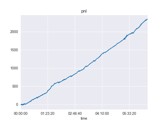
And across different runs:

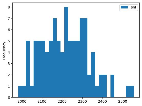
One problem of course is that the stylized model of arrival rates are too simple and do not correspond to real world markets. In the adverse selection example, if an insider wants to dump his shares, arrival rates for hits and lifts should increase and decrease respectively.

In addition, other real-world complexities like queue position and speed (and many more that I don’t have a clue about) are not modelled in this simulation, since it is purely theoretical in nature.

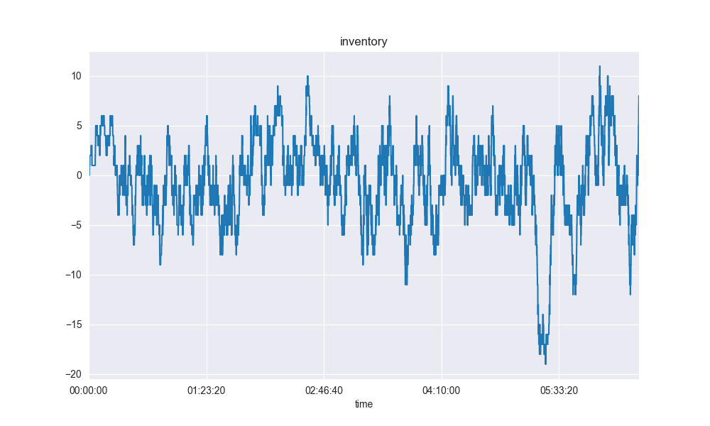
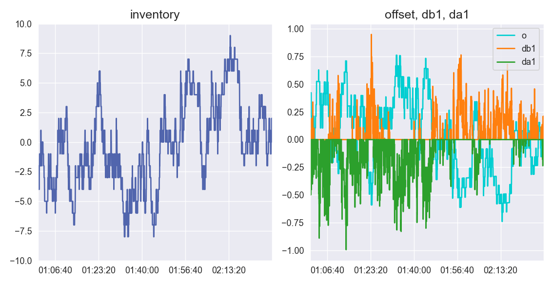
However, we can see the control theory aspect of the equations working as inventory oscillates about the zero point. Denoting db1 as the distance of the quoted bid rb distance from b1, we can zoom in on a period where inventory peaks and then troughs:

We can see that at as inventory peaks with a long position, the negative offset causes the market maker to quote more aggressive asks to clear it. Then, the makers inventory swings to short and he quotes more aggressive bids.

Another article suggested using lag 1 autocorrelation of a lagged window of price changes as a signal to stop trading as it indicates a trending market. It highlights that the A&S model corrects adverse selection after it has happened, but does not proactively avoid it.

Conclusion

To conclude, in this post, I replicate Avellaneda & Stoikov’s High Frequency Trading in a Limit Order Book. While the simulation is stylized, it still was a great learning opportunity for me.