📊 Crypto Stat Arb: Quantifying & Combining Alphas
I look at some alphas for a crypto stat arb strategy on Crypto perpetual futures on Binance. We use momentum, carry and breakout - simple price action features. I evaluate how ‘good’ they are: looking their mean returns across deciles, the info coefficients and how they decay over time. Then I combine these with ‘hardcoded’ weights to see the hypothetical returns of trading these signals frictionlessly.
Having done several paper replications and realizing they are too theoretical, I decided to implement a trading project in Python, to get familiar with basic concepts & workflow of research & backtesting a strategy. I split this two separate posts, research and backtest.
In particular, I’ve learned Pandas techniques to do quant work on cross-sectional data of a dynamic universe of stocks/tickers. My code can be found here. This project is adapted off a series by RobotJames & Kris: two well-known quants in the QuantTwit community.
Universe Selection
The data, available on their repo is of ~260 Crypto perpetual futures from 2019 to last month on Binance. It is in long form, ordered by ticker and date:

The first step is to remove Stablecoins:
url = "https://stablecoins.llama.fi/stablecoins?includePrices=true"
response = requests.get(url)
data = response.json()
stables = pd.Series([asset["symbol"] + 'USDT' for asset in data["peggedAssets"]])
perps = perps[~perps['ticker'].str.match('|'.join([f'{s}' for s in stables]))]
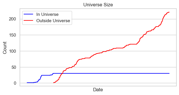
Then, the universe is selected by the top 30 perps by 30-day rolling volume. This means at any point in time, the universe of perps changes to maintain the top most liquid perps. This is done by a common workflow which repeats across the project:
universe = perps.groupby('ticker') \
    .apply(lambda x: x.assign(trail_volume=x['dollar_volume'].rolling(window=30).mean())) \
    .dropna() \
    .groupby('date') \
    .apply(lambda x: x.assign(volume_rank=x['trail_volume'].rank(ascending=False),
                              is_universe=x['trail_volume'].rank(ascending=False) <= 30))
This exposed me to the groupby-apply/transform-assign paradigm. We first groupby ticker, apply the lambda functions, using assign. We first calculate rolling 30 day dollar volume, then rank it and filter by top 30 ranks, across groups.
Simple Features
The features are:
- Breakout - closeness to 20 day highs (9.5 = new highs today/-9.5 = new highs 20 days ago)
- Carry - funding rates over last 24 hours
- Momentum - Return over last 10 days
Kris uses breakout as a time-series overlay, and carry & momentum as cross-sectional predictors of return, making the basket net long or net short, to illustrate combining xs and ts in a long-short strategy. This was purely for illustrative purposes as carry works well in the time-series as well.
features = universe.groupby('ticker') \
    .apply(lambda x: x.assign( \
        breakout=(9.5 - x['close'].rolling(20).apply(
            lambda x: x.index.values.max()-x.idxmax())).shift(),
        momo=x['close'].sub(x['close'].shift(10)).div(x['close'].shift(10)).shift(),
        carry=x['funding_rate'].shift()
        )) \
    .reset_index(drop=True) \
    .dropna()
Again, grouping by ticker and calculating the features separately within each group. We have to lag the features relative to returns. Then, we plot their distributions. Breakout is even, but momo and carry significant have positive skew.

These are scaled via z-scoring.

Then, they are bucketed into deciles for analysis. R’s ntile and Pandas qcut have different implementations, so some tweaking was needed.
scaled_features = features.groupby('date').
                  apply(lambda x:x.assign(
                  demeaned_rets = x.log_rets - x.log_rets.mean(),
                  z_carry = (x.carry - x.carry.mean())/x.carry.std(),
                  decile_carry = pd.qcut(x.carry.rank(method='first'), q=10,
                                        labels=False, duplicates='drop') + 1,
                  z_momo = (x.momo - x.momo.mean())/x.momo.std(),
                  decile_momo = pd.qcut(x.momo.rank(method='first'), q=10,
                                        labels=False, duplicates='drop') + 1,
)).reset_index(drop=True)
We do the same workflow, but qcut on ranked data to ensure equal sized buckets. At this point, this is what our scaled_features dataframe looks like:
scaled_features.columns
----
>> Index(['ticker', 'date', 'open', 'high', 'low', 'close', 'dollar_volume',
       'num_trades', 'taker_buy_volume', 'taker_buy_quote_volumne',
       'funding_rate', 'trail_volume', 'volume_rank', 'is_universe', 'rets',
       'log_rets', 'breakout', 'momo', 'carry', 'demeaned_rets', 'z_carry',
       'decile_carry', 'z_momo', 'decile_momo', 'demeaned_rets_2',
       'demeaned_rets_3', 'demeaned_rets_4', 'demeaned_rets_5',
       'demeaned_rets_6', 'demeaned_rets_7', 'log_rets_2', 'log_rets_3',
       'log_rets_4', 'log_rets_5', 'log_rets_6', 'log_rets_7'],
      dtype='object')
Exploring Features
Then, the buckets can be used to explore the features’ predictive utility, both in the xs and ts. This is done by calculating cross-sectional demeaned return (grouping by date) and time series return (grouping by ticker), then z-scoring the return to standardize it for scale. Yes I know there is some lookahead bias.
scaled_features.groupby('decile_momo').demeaned_rets.mean()
.plot(kind='bar', title='Momo decile vs next-day cross-sectional return', figsize=(10,3),rot=0)
Carry is the funding rate, where if the perp is higher priced to its coin, longs pay funding to shorts.
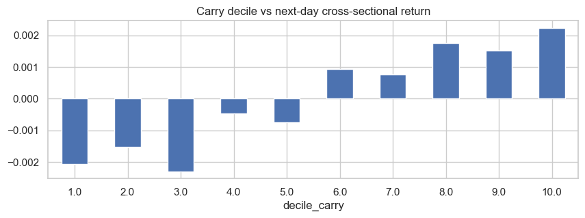
Carry deciles predict cross-sectional return very well.
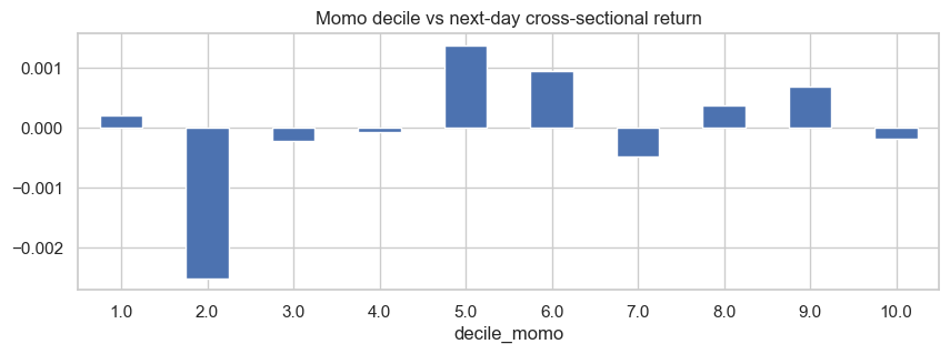
Momentum looks noisy.
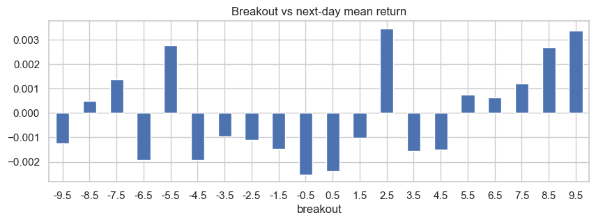
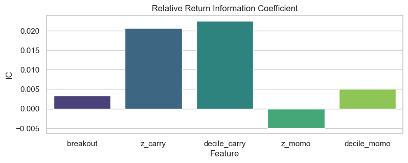
Breakout on time series return looks noisy until the 5.5 value, when there is a clear linear trend. The next step is to check information coefficients. To do so, we have to use melt to cast df into proper long form, then groupby and calculate correlation to returns. This converts the feature columns into rows.
melted_features = pd.melt(scaled_features,
            id_vars=['date', 'ticker', 'is_universe', 'demeaned_rets'],
            value_vars=['breakout', 'z_carry', 'z_momo', 'decile_carry', 'decile_momo']
            var_name='feature', value_name='value')

# Calculate Information Coefficient (IC)
ic_data = melted_features.groupby('feature')\
.apply(lambda x: pd.Series({'IC': x['value'].corr(x['demeaned_rets'])})).reset_index()
Carry clearly has the highest IC:
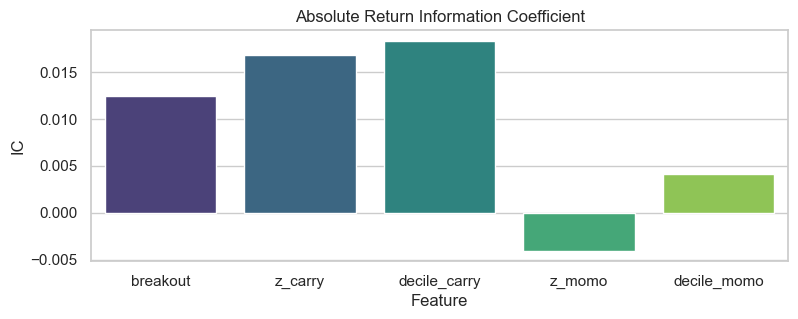
But breakout has higher IC in the ts compared to the xs:
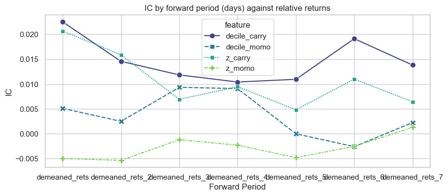
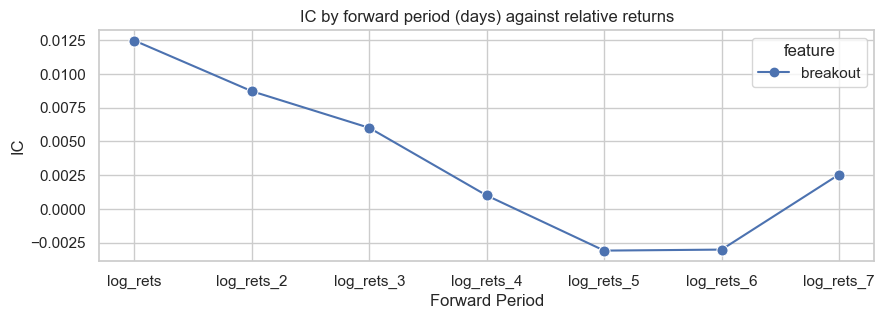
Then, the IC calculation is extended in time by calculating IC for different lookahead returns up to 7 days ahead. This is to check the signal decay, or how predictive power varies at longer horizons. This was troublesome as the df had to be melted twice.
for i in range(2,8):
    scaled_features[f'demeaned_rets_{i}'] =
    scaled_features.groupby('ticker')['demeaned_rets'].shift(-i)

# Melt the DataFrame to long format
melted_features = pd.melt(scaled_features,
                           id_vars=['date', 'ticker', 'is_universe', 'demeaned_rets']
                         + [f'demeaned_rets_{i}' for i in range(2,8)],
                           value_vars=['z_carry', 'z_momo', 'decile_carry', 'decile_momo'],
                           var_name='feature', value_name='value')

melted_melted_features = pd.melt(melted_features, id_vars=['feature','value'],
                          value_vars=['demeaned_rets']+[f'demeaned_rets_{i}' for i in range(2,8)],
                          var_name='lookahead',value_name='rets')

ic_data = melted_melted_features.groupby(['feature', 'lookahead']).apply(
    lambda x: pd.Series({'IC': x['value'].corr(x['rets'])})).reset_index()
The carry IC is sticky, which is good.
However, breakout IC decays quickly.
Lastly, correlations across the 3 signals are calculated.
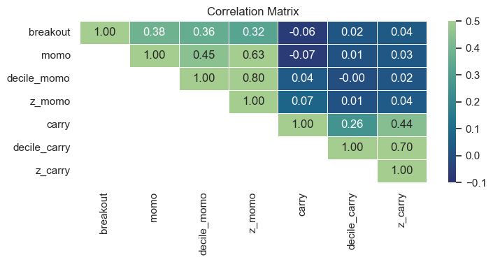
Breakout is correlated to momentum (as expected) but carry is almost uncorrelated to breakout and momentum, which is good.
Combining Signals
Next, the decile signals were to be combined into a weight. Absolute values of this weight should sum to 1 each day. Kris divides the breakout feature by two, then shifts carry and momo to put them roughly on a scale of -4.5 to 4.5.
- Since
decile_carryhas the best IC and factor plots, it is highest weighted. breakouthas moderate IC anddecile_momohas lowest IC, so they are weighted lower.
We start trading at the date when at least 3 perps are in the universe:
model_df = (
    scaled_features\
    .query('is_universe and date >= @start_date')
    .assign(
        carry_weight=lambda x: x['decile_carry'] - 5.5,
        momo_weight=lambda x: (x['decile_momo'] - 5.5),
        breakout_weight=lambda x: x['breakout'] / 2,
        combined_weight=lambda x:
        0.5 * x['carry_weight'] + 0.2 * x['momo_weight'] + 0.3 * x['breakout_weight'])
    ) \
Then, the combined weight is scaled by dividing by the absolute sum of combined weights, across all tickers, for a single day.
.groupby('date').apply(lambda x:
x.assign(scaled_weight = np.where(x.combined_weight==0,0,
            x.combined_weight/x.combined_weight.abs().sum()))) \
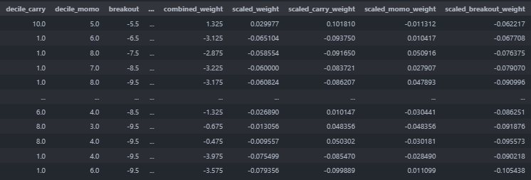
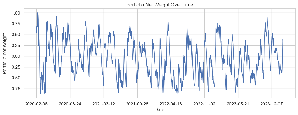
Initially, there was confusion on why the time-series feature would tilt the portfolio net long or short. However, this is because of the way the signals are calculated: momo and carry were bucketed cross-sectionally then centered, so -4.5 to 4.5 uniformly with zero mean.
Breakout on the other hand is not calculated cross-sectionally, so there is no guarantee to have zero expectation per day.
Frictionless Trading
Then, the weights are combined with returns, plotting returns to combined features with frictionless trading. This is a rough gauge of the returns, without any real-world costs. First, showing the net weights over time, with tilts due to breakout.
model_df.groupby('date').scaled_weight.sum().plot(figsize=(12,4))
Then, we can get our frictionless trading returns:
model_df['port_rets'] = model_df.log_rets* model_df.scaled_weight
model_df.groupby('date').port_rets.sum().cumsum().plot(figsize=(12,4))
plt.title('Combined Carry, Momentum, and Breakout Model on top 30 perps by volume')
plt.xlabel('')
plt.ylabel('Cumulative return')
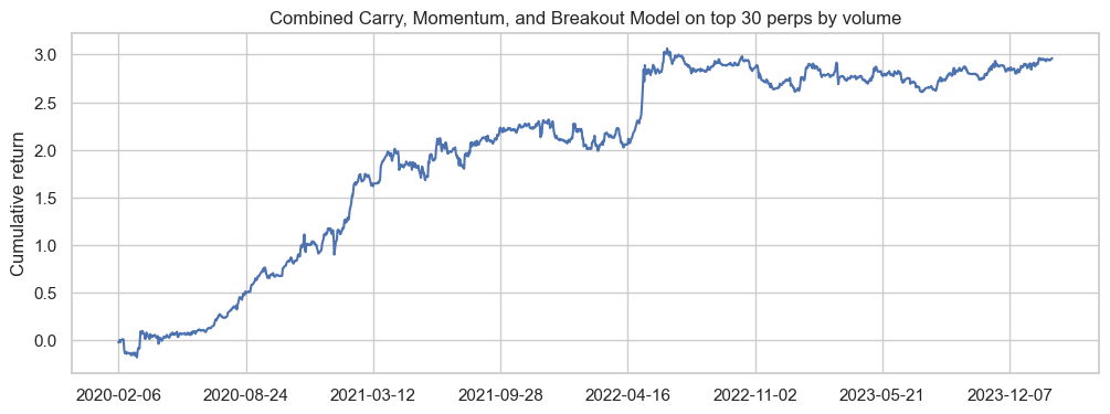
To conclude, I’ve learnt some basic quant workflows to do universe selection and signal evaluation off RobotJames & Kris’ post, which is a lifesaver because the code, data and results are there for me to evaluate if I did mine correctly. The return series is slightly different from the original post, because I flipped the sign of momentum weight (Kris used it as mean-reversion) and calculated it slightly differently (I’ve asked Kris on this and am awaiting his response).
Return Attribution
How much each factor contributes to returns separately can be examined by multiplying the factor weights by the returns - if individual factor long-short portfolios were constructed off factor deciles, with equal initial capital (I think, I could be wrong). In this case, the returns are not scaled by the weighting scheme.
.groupby('date').apply(lambda x:x.assign(
        carry_rets = x.carry_weight.mul(1)/x.combined_weight.abs().sum()
                        .mul(model_df.log_rets),
        momo_rets = x.momo_weight.mul(1)/x.combined_weight.abs().sum()
                        .mul(model_df.log_rets),
        breakout_rets = x.breakout_weight.mul(1)/x.combined_weight.abs().sum()
                        .mul(model_df.log_rets))))

model_df.groupby('date')['carry_rets','momo_rets','breakout_rets']
            .sum().cumsum().plot(figsize=(12,4))
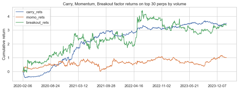
- Carry - High cumulative factor return, low volatility, but bulk of growth comes from first two years.
- Breakout - High factor cumulative return, but very volatile. Did very well in April 2022.
- Momo - Weakest cumulative return as per lowest IC.
In the next post, we can see how to combine these signals in a dynamic fashion with weights from rolling regressions to estimate expected returns. But for now, we’ve combined them in a fixed manner, with static weights, based off eyeballing our analysis above and noting the higher IC of the carry factor.
Conclusion
In conclusion, this post was my first trading project. We’ve constructed basic signals, both cross-sectional and time series, evaluated their characteristics and their returns. We’ve done so using some Pandas workflows to evaluate a dynamic universe of instruments in a cross-sectional manner.
In the next post, I adapt and translate code from RobotJames and Kris’ backtesting framework in R, Rsims, to implement the backtest in Python with trading costs and a trading buffer heuristic to reduce turnover, in place of portfolio optimization. This lets us properly evaluate the strategy with deployed capital, and compare the simple 0.5/0.2/0.3 weighting scheme to a dynamic one based off estimating expected returns with regressions.
See you in the next post!