Intuiting the Frisch-Waugh-Lovell (FWL) Theorem
So after doing some regression self-study, inspired by Chief Ridge Officer Quantymacro, I decided to write a post to consolidate some of my learnings. To give context, these guys are part of QuantTwit, a collection of quants on $\mathbb{X}$. Now if there’s anything I learned from reading $\mathbb{X}$, it’s that quants have tremendous respect for regression.
The nature of the work involves quantifying relationships between noisy, high-dim, collinear, non-stationary data, and regression fits the bill. The FWL theorem lets us spruce up our interpretation of regression in a few ways that are useful.
Disclaimer: I’m just a scrub. Please feel free to correct mistakes.
Motivating the Theorem
It’s worth noting the theorem is less related to the computational aspects of regression (no matrix decomps like SVD involved in the derivation). I’ll have a look at ridge regression and the SVD as per it’s implementation in statsmodels in a future post.
The theorem can be motivated by this question:
More generally, *all* the effects estimated by OLS are orthogonalized.
— Senior PowerPoint Engineer (@ryxcommar) October 29, 2023
Here's are 3 fun data science interview questions relating to this:
(1.) You add a new X variable to your regression, and you see that the other coefficients change. Why is that?
Intuitively, you would say “if the new predictor is correlated to other predictors, the coefficients might change”. Or conversely, “if the new predictor is uncorrelated/orthogonal to the current ones, the coefficients remain the same”.
The FWL theorem formalizes this notion. It states the individual beta of a feature in a multiple regression is a partial effect: the effect of that variable after residualising/orthogonalising out the influence of the other predictors. If we have:
\[Y=\beta_1X_1+ \beta_2X_2+\epsilon\]and want to isolate $\beta_1$, we can first regress $y \sim X_2$ and $X_1 \sim X_2$ and take their residuals, then regress first set of residuals on the second. FWL tells us the slope of this regression is our isolated beta $\beta_1$:
\[r(y \sim X_2)=\beta_1 r(X_1 \sim X_2)\]This ‘leave-one-out’, ‘residual-on-residual’ style set of regressions can be done for each beta. But why residual?
The residual of $\hat{y}{| X_2}$ is the remaining value of our $y$ that cannot be ‘explained’ by $X_2$. The residual $\hat{X_1}{| X_2}$ is the remaining part of the $X_1$ feature that is orthogonal to $X_2$. Regress the two sets of residuals, and you have found the ‘pure’ relationship between $X_1$ and $Y$ after partialling out correlations - orthogonalizing $y$ and $X_1$ w.r.t $X_2$.
So in theory, assessing a single beta in a multiple regression, one need not worry about it’s correlation to other features because it’s correlation has been partialled out! In practice, this is not the case, but that’s why ridge and SVD are used.
The Proof
I’m going to cite the proof from Gregory Gundersen’s blog in his awesome OLS article.

First, rewrite the OLS equation into partitioned form:

Relate it back to the normal equation for betas $(\textbf{X}^T\textbf{X})\hat{\beta}=\textbf{X}^T\textbf{y}$:

Expand it out. This uses the outer product to multiply the first two matrices together, then transform the beta vector to give two equations.

Solve for $\hat{\beta_1}$:

Substitute this expression for $\hat{\beta_1}$ into the second equation:

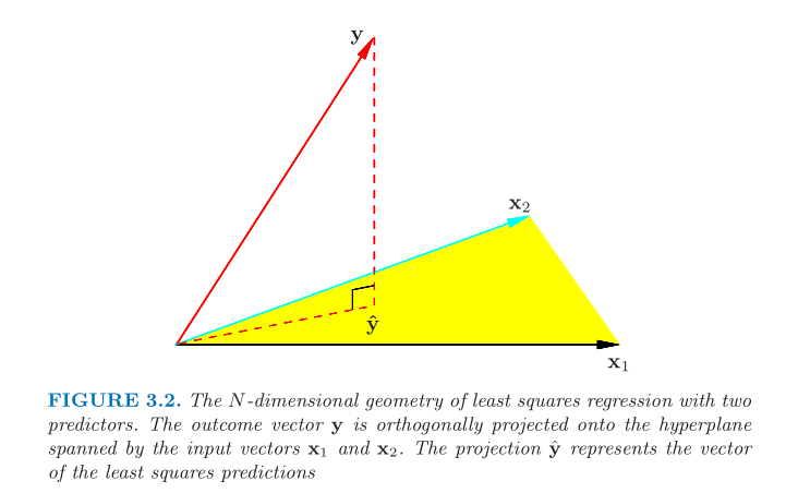
Define the hat and residual maker matrices. The hat matrix orthogonally projects the endogenous vector onto the column space of the design matrix. Hastie & Tibshirani illustrate this in §3.2.3 of ESL which is the first image in this post. The hat and residual maker matrices are orthogonal.

Put them into the equation and solve for $\hat{\beta_2}$ in terms of residual-on-residual regression.

Rearrange the terms:

This expression is the normal equation for regressing $\textbf{y}$ on $\textbf{X}_2$ but with $\textbf{M}_1$ in front of $\textbf{y}$ and certain $\textbf{X}_2$ terms. Why not in front of the first $\textbf{X}_2$? Because $\textbf{M}_1$ is an orthogonal projection aka $\textbf{M}=\textbf{M}^2$ and also orthogonal so $\textbf{M}=\textbf{M}^T$.
So the residual-on-residual idea of FWL can be expressed in terms of the residual maker matrix $\textbf{M}_1\textbf{y} = \textbf{M}_1\textbf{X}_2\hat{\beta_2} + \textbf{e}$.
Why Is This Useful
But who cares? Why is this useful? Here are some reasons:
- The interpretation of individual $\hat{\beta}_i$ after partialling out correlation effects.
- Relates geometry (orthogonalisation/residualisation) to removing correlation (assuming linear relationship).
- Viewing
sm.add_constant(X)to the design matrix for an intercept as partitioned regression where $\textbf{X}_1=\textbf{1}$, equivalent to demeaning.
Tree-based ML models (rf, xgb, etc) don’t have this neat interpretation of coefficients! It would be interesting to compare feature importances of a tree-based model like xgboost to the betas from linear regression both fit on the same data.
Essentially, subtracting the mean, i.e. centering the vector, is the same thing as orthogonalizing with respect to a constant term.
— Senior PowerPoint Engineer (@ryxcommar) October 29, 2023
This is how we get to Var(x), and not just simply x².
Sweet! We now see how (X'X)⁻¹ and 1/Var(x) are related.
Again, this derivation is from Gundersen. In simple regression, the intercept is the difference of two means, effectively de-meaning the target and predictor:
\[\hat{\alpha}=\bar{y}-\hat{\beta}\bar{x}\]Why would you want an intercept? This image from Gundersen’s blog shows why:
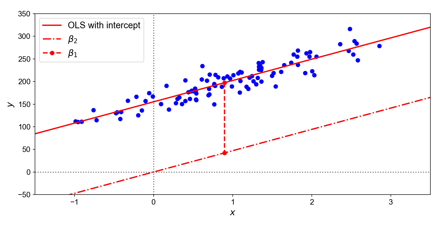
So you do a parallel shift of your regression slope upwards by a constant coefficient to account for differences in means. Anyway, in the multiple regression case, we set $\textbf{M}_1$ where $X_1=\textbf{1}$ and compute $\beta_1$
\[\textbf{y}= \textbf{1}\beta_1 + \textbf{X}_2\beta_2 +\textbf{e}\]The hat matrix $\textbf{H}_1$ expands out to become a $1/N$ matrix. Note an error in the picture, it should be $(\textbf{1}^T\textbf{1})^{-1}$.

This $\textbf{1}$ hat matrix when applied to the design matrix effectively produces column-wise means in every entry. To see this, use the inner product view of matrix multiplication.

And it acts on the design matrix and the vector. So our $\hat{\beta}_2$ is effectively a demean and a regression:

Now use the equation for $\beta{1}$ that was derived earlier with $\textbf{X}_1=\textbf{1}$. And of course, the difference-in-means is captured in the $\hat{\beta{1}}$ as the hat matrix demeans the terms, and we see the intercept as a generalized case as the simple OLS intercept.

I think it’s worth understanding what the intercept does, especially later in the case of multilevel regression/mixed effects models where you can have random intercepts, random slopes or both - see 0xfdf’s post on using multilevel regression to create a signal.
And in commodities, there might be lots of chances to use mixed effects models (e.g predict some quantity across countries or different geographical areas).
The Case Study
Let’s look at a made-up example to see the FWL theorem in action. This example is purely for illustration purposes. Suppose we want to predict attractiveness from height and face, and these quantities are all z-scores, and the true relationship is linear:
\[Attr \sim 1 Face + 0.4 Height + \epsilon\]That is, face contributes to attractiveness ~ twice that of height. However, face is highly collinear to height (0.7). We can simulate this dataset.
import numpy as np
import pandas as pd
import statsmodels.formula.api as smf
np.random.seed(69)

n = 50
rho = 0.7
beta1, beta2 = 1, 0.4

cov = np.array([1,rho,rho,1]).reshape(2,2)
mu = np.array([0,0])

exog = np.random.multivariate_normal(mu, cov, size=n)
endog = beta1 * exog.T[0] + beta2 * exog.T[1] + np.random.normal(0, 0.1, size=n)

df = pd.DataFrame(np.column_stack((exog, endog)), columns=['face', 'height', 'attr'])

hf = smf.ols('height ~ face', data=df).fit()
fh = smf.ols('face ~ height', data=df).fit()
ah = smf.ols('attr ~ height', data=df).fit()
af = smf.ols('attr ~ face', data=df).fit()
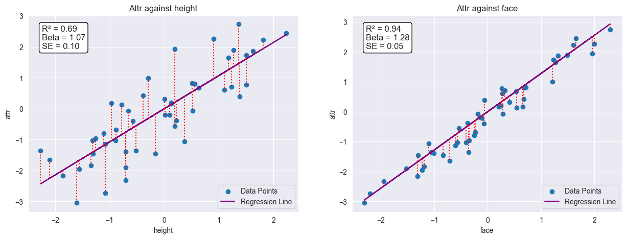
Plotting individual simple regressions of face and height, we see the individual betas are over-estimated because of the correlation between the two features.
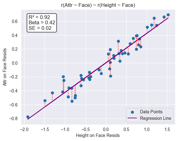
Now let’s isolate our height beta. We orthogonalize height on face and attractiveness on face.
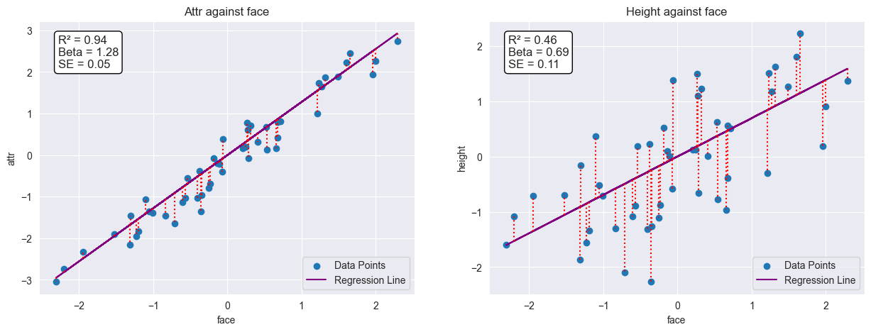
We are left with the residuals, the variation of height and attractiveness that are orthogonal to face.
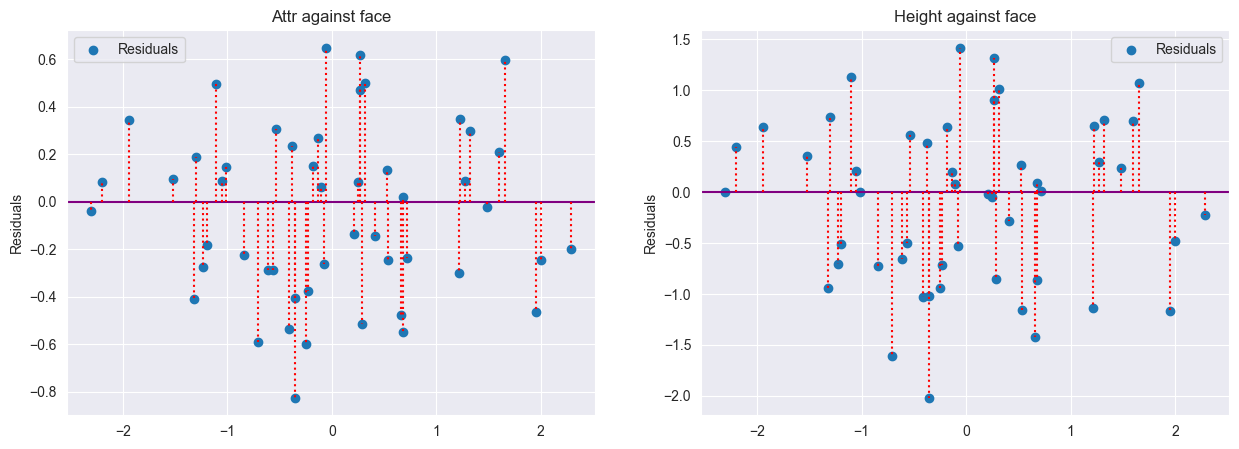
Regressing the orthogonalized (w.r.t face) variables (residuals), demeaned, against each other, we recover the original height beta in the true relationship ($\pm$ the standard error):
Further Stuff
That concludes this short article! For further investigation, I’d very much like to know how this works …
"Question 8: Describe the difference between iterated regression and matrix decomp (rotation) to transform an N x M matrix so that each of the N columns is pairwise orthogonal."
— fdf (@0xfdf) July 21, 2024
But I’ll work on that slowly.
For now, the FWL theorem provides us with essential intuition about key facets of multiple regression without going into any implementation details yet.
To understand FWL is to understand a key intuition of what multiple regression is actually doing.
— Senior PowerPoint Engineer (@ryxcommar) June 26, 2023
I’ll look at ridge regression (from QM articles of course) and how statsmodels implements it under the hood with SVD. In particular, to see how it deals with collinearity, and how to determine regularization strength.